Goal

Rectify a weakly calibrated stereo image pair — only the fundamental matrix known, no intrinsics, extrinsics, or projection matrices — so that corresponding points fall on corresponding rows, for arbitrary camera motion. Input: the two source images plus the oriented fundamental matrix $F$ between them, obtained from the usual $\geq 7$ point correspondences plus one additional correspondence used solely to fix orientation. Output: two resampled images built by direct, nonlinear warping of the originals, with no pixel of either source dropped and an output size bounded purely by the source dimensions. The construction handles the case a planar-homography rectification cannot represent at all: an epipole lying inside either image, which under a mapping-to-infinity homography would force an unbounded output.

Algorithm

Let $w \times h$ denote the pixel dimensions of a source image; each source image is bounded by its own $w, h$ (the two images need not share dimensions). Let $e, e'$ denote the epipoles of image 1 and image 2 — the right and left null spaces of $F$ , $Fe = 0$ and $F^\top e' = 0$ . Let $l$ and $l'$ denote a corresponding pair of epipolar lines, with $l' \sim Fm$ for a point $m$ in image 1. Let $H$ denote the homography used only to transfer epipolar lines between the two images — not a rectifying homography in the planar-rectification sense, since it is never applied to warp pixels directly. Let $a$ denote an arbitrary vector used to build $H$ , subject to $\det H \neq 0$ . Let $\theta$ index angular sectors (rows of the rectified output) and $r$ index radial distance from the epipole within a sector.

Definition

Epipolar-line-transfer homography

Transfers an epipolar line of one image to its corresponding line in the other; it is not used to warp pixels.

H = [e']_\times F + e' a^\top, \qquad \det H \neq 0, \qquad l' \sim H^{-\top} l.

Definition

Orientation sign function

Fixes which half of each epipolar line in image 1 matches which half in image 2, removing the sign ambiguity that an unoriented $F$ leaves undetermined.

f_l(m) = l^\top m, \qquad m = [x\ y\ 1]^\top.

For one known correspondence $(m_0, m_0')$ beyond the $\geq 7$ used to estimate $F$ , the sign of $a$ is chosen so that $f_l(m_0)$ and $f_{l'}(m_0')$ agree. Every other epipolar line's residual ambiguity is then a strictly positive scale factor, splitting each line into a positive half and a negative half that consistently correspond across the two images.

Definition

Output size bound

Guaranteed independently of where the epipole sits or how well $F$ is conditioned — the bound depends only on the source dimensions.

h_{\text{out}} \le 2(w+h), \qquad w_{\text{out}} \le \sqrt{w^2+h^2}.

Procedure

Algorithm

Polar rectification

Input: Two images with dimensions

w \times h

each; the oriented fundamental matrix

F

between them.

Output: Two resampled images with corresponding points on corresponding rows; a per-row lookup table mapping each rectified row back to its source epipolar line.

Estimate $F$ from $\geq 7$ point correspondences, then fix its orientation using one additional correspondence via the sign function $f_l$ .
Build the transfer homography $H = [e']_\times F + e' a^\top$ for an arbitrary $a$ with $\det H \neq 0$ , and use it to transfer epipolar lines between the images via $l' \sim H^{-\top} l$ .
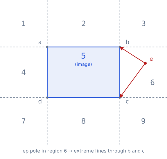
In each image independently, classify the epipole's position into one of nine regions relative to the image rectangle's corners and locate the extreme epipolar lines — the ones touching the corners.
Transfer the second image's extreme lines into the first image via $H$ and intersect them with the first image's own extreme lines to obtain the angular range common to both images.
Build the rectified image row by row within that common range: each row is one angular sector (one half epipolar line), and the radial coordinate $r$ along the line is copied unchanged, with no resampling along $r$ .
Choose the angular step $\Delta\theta$ between consecutive rows from a congruent-triangle construction on the worst-case pixel, always located on the image border opposite the epipole; repeat the construction in the other image, transfer its result back, and use the smaller of the two candidate steps so neither image loses a pixel.
If the epipole lies inside the image, start the sweep from an arbitrary epipolar line and continue past $360°$ , overlapping by the size of the stereo-matching window to avoid a seam at the wrap-around boundary.
Record each row's epipolar-line endpoint distances in a lookup table for the inverse mapping back to the source images, interpolating for sub-pixel accuracy, and reconstruct a full image radially — filling all pixels between two consecutive epipolar lines at once — rather than one lookup per output pixel.

Implementation

The homography construction, orientation check, and per-row step rule in Rust:

type Vec3 = [f64; 3];
type Mat3 = [[f64; 3]; 3];

/// Epipolar-line transfer homography H = [e']_x F + e' a^T (det H != 0);
/// transfers lines via l' ~ H^-T l.
fn epipolar_homography(f: Mat3, e_prime: Vec3, a: Vec3) -> Mat3 {
    let skew: Mat3 = [
        [0.0, -e_prime[2], e_prime[1]],
        [e_prime[2], 0.0, -e_prime[0]],
        [-e_prime[1], e_prime[0], 0.0],
    ];
    let mut h = [[0.0; 3]; 3];
    for i in 0..3 {
        for j in 0..3 {
            let cross_f: f64 = (0..3).map(|k| skew[i][k] * f[k][j]).sum();
            h[i][j] = cross_f + e_prime[i] * a[j];
        }
    }
    h
}

/// Signed line-membership function f_l(m) = l^T m, m = [x y 1]^T. Orientation
/// is fixed by requiring this sign to agree, for one known correspondence, across both images.
fn line_side(l: Vec3, x: f64, y: f64) -> f64 {
    l[0] * x + l[1] * y + l[2]
}

/// Candidate step from the congruent-triangle construction: the worst-case
/// pixel sits at border point `b` (opposite the epipole), bracketed by `a`
/// (previous) and `c` (next). The step used is the minimum of this value
/// and the candidate transferred back from the other image.
fn candidate_step(a: (f64, f64), b: (f64, f64), c: (f64, f64)) -> f64 {
    let dist = |p: (f64, f64), q: (f64, f64)| ((p.0 - q.0).powi(2) + (p.1 - q.1).powi(2)).sqrt();
    dist(b, c) / dist(a, c)
}

/// Guaranteed bounds on rectified output size, from source dimensions alone.
fn output_size_bound(w: f64, h: f64) -> (f64, f64) {
    (2.0 * (w + h), (w * w + h * h).sqrt())
}

Remarks

The output-size bound is combinatorial, not data-dependent: $2(w+h)$ and $\sqrt{w^2+h^2}$ depend only on the source dimensions, unlike planar rectification's output size, which grows without bound as the epipole approaches the image.
The row-by-row polar construction is a nonlinear warp: the rectified images are non-rectangular and visibly distorted compared to a planar-homography-rectified pair.
Orientation is a discrete sign choice fixed from one extra point correspondence beyond the $\geq 7$ used for $F$ ; a mismatched seed correspondence flips the positive/negative convention for the whole image.
All operations are carried out directly in the two 2-D image planes; no 3-D reconstruction step is involved, in contrast to cylindrical-rectification schemes that operate in 3-D and size the output from a single worst-case cylinder diameter.
Rectification bounds the output size but does not remove the epipole as a singularity for downstream depth estimation when the epipole lies inside the image.
The comparison against planar rectification methods is hosted on the survey concept page: see Stereo rectification — decision table.

References

M. Pollefeys, R. Koch, L. Van Gool. A Simple and Efficient Rectification Method for General Motion. ICCV, 1999, pp. 496–501. doi.org/10.1109/ICCV.1999.791262
H. C. Longuet-Higgins. A computer algorithm for reconstructing a scene from two projections. Nature 293:133–135, 1981.

Pollefeys Polar Rectification

Goal

Algorithm

Procedure

Implementation

Remarks

References

Prerequisites

Compared with