Goal

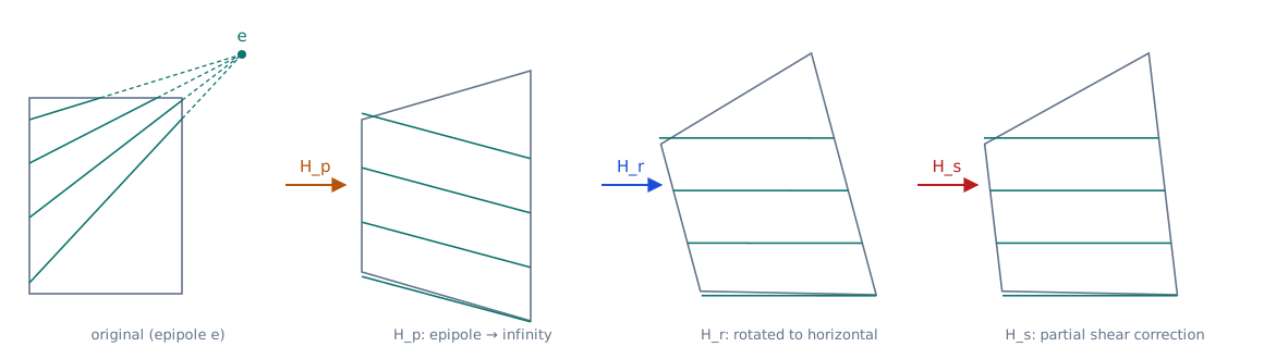
Rectify a calibrated or uncalibrated stereo pair given the fundamental matrix $F$ (or essential matrix $E$ for a calibrated pair) relating the two views. Input: two images $I$, $I'$ of a static scene satisfying the epipolar constraint $\mathbf x'^T F\,\mathbf x = 0$ for every correspondence $\mathbf x \leftrightarrow \mathbf x'$, with $F$ assumed known in advance. Output: a pair of homographies $H$, $H'$ such that the rectified points $\hat{\mathbf x} = H\mathbf x$, $\hat{\mathbf x}' = H'\mathbf x'$ satisfy a canonical rectified epipolar geometry — both epipoles map to a common point at infinity and corresponding points fall on identical scanlines. Each homography is factored as $H = H_s H_r H_p$: a projective component chosen from a quantifiable 2D distortion-minimization criterion, a similarity component that aligns epipolar lines with the horizontal axis, and a shearing component that spends the remaining degrees of freedom to further reduce distortion.

Algorithm

Let $\mathbf x = (u, v, 1)^T \in I$ and $\mathbf x' = (u', v', 1)^T \in I'$ denote homogeneous image coordinates. Let $F$ be the known, rank-2 $3\times3$ fundamental matrix satisfying $\mathbf x'^T F\,\mathbf x = 0$. Let $\mathbf e$, $\mathbf e'$ denote the epipoles, defined by $F\mathbf e = \mathbf 0$ and $F^T\mathbf e' = \mathbf 0$. Let $\mathbf i = (1, 0, 0)^T$ denote the canonical rectified-epipole direction, and $[\mathbf i]_\times$ its cross-product matrix.

Each rectifying homography is a product of three special-purpose transforms, applied to the corresponding image in this order:

$H_p$ (and $H_p'$) is a projective transform sending the epipole to a point at infinity. The map to infinity admits a one-parameter family of solutions, parameterized by a free direction $z$ shared between the two images. The per-image epipolar-line normal induced by $z$ is

Minimizing this joint criterion is a nonlinear problem: its stationary condition reduces to a degree-7 polynomial in the single free scalar of $z$, solved by iterative root-finding. The seed for the iteration comes from solving the two single-image terms separately in closed form — each single-image ratio is a generalized-eigenvalue problem, $A_{\text{img}} = D^TD$, whose maximizer is the top eigenvector of $D^{-T}BD^{-1}$; the average of the two single-image solutions is reported to lie close to the joint optimum, though without a proven bound.

$H_r$ (and $H_r'$) is a similarity transform that rotates the now-infinite image of the epipole into alignment with $\mathbf i$, together with a shared vertical offset that aligns the two images' scanlines exactly. The pair $H_p H_r$, $H_p' H_r'$ already satisfies the rectified epipolar geometry above; the remaining horizontal degrees of freedom are still free at this point.

$H_s$ (and $H_s'$) is a shearing transform, affecting only the $u$-coordinate of a point and therefore leaving rectification undisturbed. It spends the remaining freedom to preserve perpendicularity and aspect ratio of the quadrilateral formed by the midpoints of the image's four edges — a system of two simultaneous quadratics in the shear parameters, solved via the curve-intersection method of Manocha and Demmel (1994), with a sign ambiguity resolved by preferring the positive root. In general $H_p$ is projective, so the affine shear cannot fully undo its distortion; it satisfies only these two constraints, not a general distortion minimum.

Procedure

Implementation

The epipolar-line-normal parameterization (Eq. 8) and the final per-image homography composition in Rust:

type Vec3 = [f64; 3];
type Mat3 = [[f64; 3]; 3];

/// Cross-product matrix [v]_x.
fn cross_matrix(v: Vec3) -> Mat3 {
    [
        [0.0, -v[2], v[1]],
        [v[2], 0.0, -v[0]],
        [-v[1], v[0], 0.0],
    ]
}

fn mat_vec(m: Mat3, v: Vec3) -> Vec3 {
    let mut out = [0.0; 3];
    for i in 0..3 {
        out[i] = m[i][0] * v[0] + m[i][1] * v[1] + m[i][2] * v[2];
    }
    out
}

fn mat_mul(a: Mat3, b: Mat3) -> Mat3 {
    let mut c = [[0.0; 3]; 3];
    for i in 0..3 {
        for j in 0..3 {
            c[i][j] = (0..3).map(|k| a[i][k] * b[k][j]).sum();
        }
    }
    c
}

/// w = [e]_x z (image I), w' = F z (image I').
fn epipolar_line_normals(e: Vec3, f: Mat3, z: Vec3) -> (Vec3, Vec3) {
    (mat_vec(cross_matrix(e), z), mat_vec(f, z))
}

/// H = H_s H_r H_p, applied per image.
fn rectifying_homography(h_s: Mat3, h_r: Mat3, h_p: Mat3) -> Mat3 {
    mat_mul(mat_mul(h_s, h_r), h_p)
}

The projective-distortion criterion (Eq. 11), its degree-7 stationary-point solve, and the shear-parameter quadratics are omitted: they require a generalized-eigenvalue routine and a polynomial root-finder not expressible in a self-contained snippet.

Remarks

• Works identically for calibrated pairs (fundamental matrix specializes to the essential matrix) and uncalibrated pairs; the method assumes $F$ is already known and does not estimate it.
• Zero projective distortion is unattainable in general except when the epipole starts at infinity, and the shear stage cannot fully undo the projective component's distortion — it satisfies only the perpendicularity and aspect-ratio constraints, not a general minimum.
• The joint two-image projective-distortion criterion has no closed form: it requires an iterative degree-7 polynomial root-find, with no proven bound on distance from the optimum.
• Because the projective component is constructed to send the epipole to a point at infinity, an epipole located inside the image frame drives part of the rectified image toward infinity, forcing cropping in practice; an epipole outside the image frame does not have this problem.
• Comparison with other rectification approaches is on the stereo rectification decision table.

References

1. C. Loop, Z. Zhang. Computing Rectifying Homographies for Stereo Vision. IEEE CVPR, 1999. pdf