1. Introduction

Calibrating visual sensors in challenging setups is part of my job. In practice this means multi-camera rigs, significant lens distortion, tilted optics, and images where corner localization is expected to be both accurate and stable. At some point it became clear to me that the OpenCV calibration toolset was not good enough for my use cases: not only in accuracy, but also in performance, robustness, and control over the full pipeline. That is how I started building my own calibration stack, beginning with chessboard target detection.

The first question was simple: how should one detect chessboard corners?

Classical detectors such as Harris, Shi-Tomasi, or FAST are designed to react to corner-like structures in general. That is exactly why they are broadly useful, and also why they are not ideal here. A chessboard corner is more specific than a generic corner: locally, it forms an X-junction with an alternating black-white arrangement. Since this structure is known in advance, it is better to encode it directly in the detector.

(OpenCV’s chessboard detector follows a different route: it starts from segmenting black squares and then derives corners from the recovered geometry. That works well, but it couples the problem to global board structure and requires the whole pattern to be visible, which is not acceptable in my case.)

Bennett and Lasenby proposed an elegant, robust, and efficient detector, ChESS (Chess-board Extraction by Subtraction and Summation), designed specifically for chessboard-like X-junctions. In my view, this idea deserves more attention in the vision community. In this post, we will look at ChESS in some detail, closely following the original paper. By the end, you should have a clear picture of how my implementation of ChESS works.

2. The ChESS response

The ChESS detector computes a score for each pixel. Pixels that lie on X-junctions receive a large score; pixels on edges, stripes, or textured regions receive a small one.

The core idea is to sample a ring of 16 pixels around the pixel of interest, at radius 5:

Radius 5 is chosen because it is the smallest radius at which these 16 samples can be arranged with nearly uniform angular spacing. At the same time, it keeps the detector local.

The sum response

A chessboard corner creates an alternating pattern on the ring: bright, dark, bright, dark. This means that opposite samples have similar intensity, while samples rotated by $90^\circ$ have opposite intensity. This leads to the basic combination

When the ring is centered on a true X-junction, this quantity becomes large in magnitude. Summing the four rotated versions gives the sum response:

This already captures the main signal of a chessboard corner. But it is not enough, because other structures can also produce a strong response. In particular, two false-positive families matter here: edges and narrow stripes.

Rejecting edges

Consider the edge case shown below.

For an ideal straight edge, $SR$ is exactly zero, because the sampling pattern lacks the alternating structure of a chessboard corner and the corresponding terms cancel. Real images, however, are affected by noise, blur, discretization, and centering errors, all of which can break this symmetry and produce a spurious response. This motivates the introduction of a separate edge-sensitive term.

The key observation is that on an edge, opposite samples often have opposite brightness. This leads to the diff response:

This term is large on edges and relatively small on true chessboard corners. So the natural next step is to penalize the sum response by the diff response:

This gives exactly the desired behavior: true chessboard corners retain a strong response, while edge-like structures are suppressed.

Rejecting stripes

The second false-positive case is more subtle. A narrow stripe can produce almost the same ring pattern as a true corner.

This is an important limitation: the ambiguity cannot be resolved from the ring samples alone. The missing information lies near the center of the pattern, as illustrated below.

The solution is to compare two averages:

• the average intensity over the five central pixels, denoted $I_{center}$
• the average intensity over the 16 ring samples, denoted $I_{ring}$

Their difference defines the mean response:

For a true X-junction, the center and ring averages are similar, so $MR$ is small. For a narrow stripe, they differ significantly, which makes $MR$ large.

The final ChESS response is therefore

The coefficient 16 is chosen so that narrow stripes produce a response that stays safely below zero.

With this term included, the detector distinguishes true chessboard corners from the main false-positive structures discussed above. The final expression remains remarkably compact: it requires only a small fixed number of intensity reads and arithmetic operations per pixel. That compactness is what makes the detector cheap to run and easy to vectorize.

The demo below shows how the ChESS score behaves on three characteristic patterns: a true corner, an edge, and a narrow stripe.

3. From heat map to features

The response defined above gives a dense heat map, but in practice we need actual feature points.

The next step is standard: compute the response image, suppress negative or weak values, and apply non-maximum suppression to retain only local maxima. This converts a dense pixel-wise score into a sparse set of corner candidates at pixel precision.

Pixel precision, however, is rarely sufficient. Good feature localization is typically expected to reach roughly one tenth of a pixel. This calls for an additional subpixel refinement step.

The ChESS response is usually quite symmetric around a true corner. Because of that, even a simple center-of-mass refinement works well. Take a small window around the candidate, for example $5 \times 5$ pixels, and compute the centroid of the local response distribution:

where the sums run over all $(x, y)$ in the refinement window, and $w(x,y)$ is the ChESS response at pixel $(x, y)$.

In my implementation, I use several classical subpixel refinement methods, as well as a CNN-based refiner. That part deserves a separate discussion, so I will return to it in another post.

4. Corner orientation

The original paper also discusses corner orientation, but in a quantized form: it assigns each detected corner to one of eight orientation bins.

In my implementation, I instead compute a continuous orientation as an additional descriptor.

This is done after detection and subpixel refinement. For each corner, the original grayscale image is sampled on a 16-point ring around the refined subpixel location, using bilinear interpolation. The 16 sampled values form a signal on the ring; subtracting their mean removes the constant offset and leaves the angular variation that carries the orientation information.

The idea is similar to a Fourier transform: the ring signal is decomposed into repeating angular patterns. For a chessboard corner, the relevant pattern repeats twice during one full turn around the ring. Its phase gives the local corner orientation.

This leads to

Here $s_i$ are the ring samples, $\bar{s}$ is their mean, and $\phi_i$ is the angle of the $i$-th sample on the ring. The complex value $M$ tells us how strongly this twice-per-turn pattern is present and at which angle it is aligned.

The orientation is defined modulo $\pi$, since reversing the direction gives the same line.

This orientation becomes useful later when reconstructing board structure and filtering out geometrically inconsistent detections.

5. ChESS in Rust

The Rust implementation lives in this repository. You can install it with cargo:

cargo add chess-corners

and use it like this:

use chess_corners::{ChessConfig, find_chess_corners_image};
use image::ImageReader;

let img = ImageReader::open("board.png")?.decode()?.to_luma8();
let cfg = ChessConfig::single_scale();
let corners = find_chess_corners_image(&img, &cfg);
println!("found {} corners", corners.len());

Python bindings are also available on PyPI:

uv pip install chess-corners

Usage is similarly straightforward:

import numpy as np
import chess_corners as cc

img = np.zeros((128, 128), dtype=np.uint8)
cfg = cc.ChessConfig.single_scale()
corners = cc.find_chess_corners(img, cfg)

The implementation includes features that are not discussed in this post, such as multiscale detection using an image pyramid, and exposes a number of configuration parameters. In most practical cases, however, the default settings should work well.

The image below shows an example input used for benchmarking:

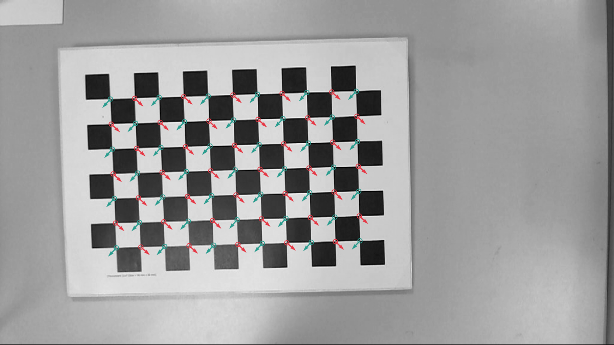
One notable property of this detector is its speed. Detecting features in the image above ($1024 \times 576$ pixels) takes about 1.2 ms on my MacBook Pro with an M4 chip, with the rayon and simd features enabled. On the same image, OpenCV’s pixel-precise Harris detector takes about 3.9 ms, while findChessboardCornersSB takes about 115 ms.

The last comparison is only partial, because findChessboardCornersSB is a full chessboard detector, while ChESS here covers only the corner-detection stage. A full chessboard detector built on top of ChESS takes less than 4 ms on the same image. I will return to that in a future post. The implementation is available in calib-targets-rs.

A more detailed discussion can be found in the performance report.

6. Final thoughts

The main advantage of ChESS is that it is both simple and designed specifically for chessboard corners:

• It provides orientation information for each corner. This is very useful for recovering global structure and rejecting false positives.
• It does not require committing to a global board model at the response stage. This makes it attractive in the presence of strong lens distortion and other difficult imaging conditions.
• It produces an interpretable quality score, which gives direct control over detection sensitivity and the recall-precision tradeoff.
• It is computationally simple. That simplicity translates directly into fast implementations, parallel execution, and clean multiscale extensions.

Overall, ChESS is a simple and practical detector. It is fast, robust, and well suited to pipelines that need millisecond-scale corner detection under strong lens distortion.